Visualization

The goal of the CodeCharta visualization is to make code quality more accessible to everyone. We use the city metaphor and represent each file in your source code with a building. This allows user to grasp complex metrics, even without knowing what they are in detail. This also provides a big picture view of code to experienced professionals and allows them free exploration of the code files and their metrics.

We won’t sugar coat it, the visualization can look a bit daunting at first. This is what you will find, once you open the web visualization:

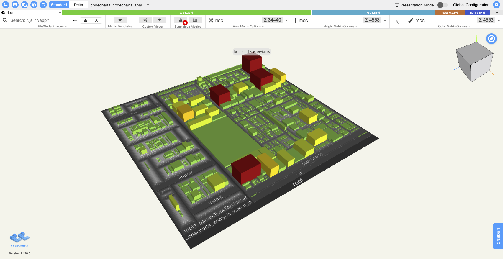
The main focus is the city-style map. Each building in it has the attributes size, height and color, which are selectable via drop down menus and can each represent a different metric. This way the visualization allows users to contrast multiple metrics at the same time. The default settings for these metrics looks like this:

• size =rloc (real lines of code)
• height =complexity (cyclomatic complexity)
• color =complexity (cyclomatic complexity)

Note that the available metrics are tied to the cc.json used to load the map. Depending on which parser of our ccsh tool was used to generate the map, different metrics might be available. For more information on what these names mean and which parsers produce which metrics, view the list of available tools in analysis.

Exploring Code with CodeCharta

Let us take a look at how CodeChart can be used to explore code metrics by playing around with the web visualization.

After you open it, you will see a map similar to the screenshot above. You can rotate the map by holding left-click and move the map by holding right-click. For more detailed controls, see User Controls.

After clicking on a building of your choice (maybe one of the big red ones looks interesting) you will see the filename, the path to the file, the currently selected metrics (called primary metrics) and all available metrics (secondary metrics). Now we can see all kinds of numbers, but what can we do with them?

Let’s look at an example. Per default, the size is set to rloc (real lines of code), which represents how long a file is. The other two metrics are set to complexity, which (you guessed it) represents how complex a file is. Now lets take a look at the biggest, tallest, reddest building. Without additional knowledge you can easily identify the most complex file in the whole codebase, no matter how big it is. But can do we do with this information?

Try changing the color metric to line_coverage. Now the color of some buildings has changed while their height stayed the same. The height and the color now represent two different metrics. Through this, we have now combined the complexity of a file with how thoroughly it is tested. A building that is tall and green might be complex, but has enough tests to achieve a high line coverage. However, if we spot a tall red building, we have found a complex file, that is barely tested. Now think about the most complex building you found earlier, is it still red because it also has a low code coverage? If it is, this gives you another indication that it needs improvement.

If it is green then you could change the color metric to number_of_authors (if that metric is available in your map). A building that is complex, has low code coverage and only one author can be very problematic, because that code is only known by one person. On the other hand a building that has many authors can be problematic because it is now a coordination bottleneck: apparently everyone needs to modify that file.

Combining metrics

This is just one example how you can explore your source code. Once you get a feel for the metrics, you might decide to combine different metrics. We usually leave the size metric locked to the real lines of code metric though. That ensures the buildings are always in the same place, even when you change height and color.

Depending on the tools you used to generate your map you might also be able to view the edges between buildings (check out the tools individual pages to see if they can generate edge metrics). Edges show connections between your files and can take many forms. For example the metric pairingRate tells you that when file A is committed, file B is also in that same commit. Now there is an edge between building A and building B, an unidirectional relationship. But file B might also show up in commits that don’t include file A. No edge between building B and building A then.

You can see the building with most edges because purple edges leave and cyan edges enter. When you hover over a building with edges you can see exactly where they lead or are coming from. Edges that stretch over the whole map might indicate a problem because buildings that are connected should usually be put in the same package in your source code.

Icons by fontawesome